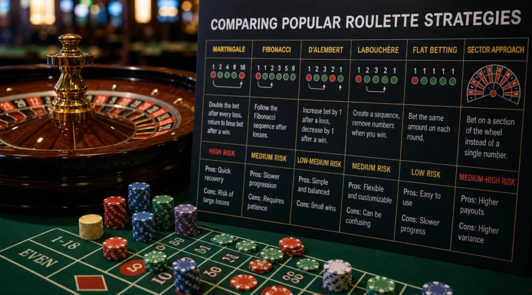
Practical, side‑by‑side comparison of popular roulette strategies: Martingale, Fibonacci, D’Alembert, Labouchère, flat betting and sector approaches

Clear guide to roulette strategies: what this comparison shows
This article explains common roulette strategies and what a player should realistically expect. It compares how Martingale, Fibonacci, D’Alembert, Labouchère, flat betting and sector/visual approaches work, shows simple sample bet sequences, gives the basic math behind each method, and highlights expected outcomes, bankroll requirements and practical risks in both online and land‑based play. Readers will learn that while systems change how you size bets, they do not change roulette’s underlying house edge.
Roulette math basics every strategy depends on
Understanding a few core probabilities makes it easy to evaluate systems. European roulette has 37 pockets (0–36); American roulette adds 00 (38 pockets). Common facts:
- Even‑money bets (red/black, odd/even) pay 1:1 but win slightly less than 50% of the time: European p = 18/37 ≈ 48.65%; American p = 18/38 ≈ 47.37%.
- Expected value (EV) for any fixed bet is negative and equals -house edge × bet. For European roulette the house edge is 2.70% (EV ≈ -0.027 per $1); for American it’s 5.26%.
- Probability of N consecutive losses on an even bet (European): q^N where q = 19/37 ≈ 0.5135. For example, six losses in a row happen with probability (19/37)^6 ≈ 1.8% — low but meaningful over many sessions.
Key takeaway: no betting system alters EV. Systems change variance and the shape of wins/losses, and they can increase the risk of large drawdowns or ruin when table limits and finite bankrolls are considered.
How the main roulette strategies work (quick primer and sample sequences)
The following explains each system’s rules, a short sample sequence and immediate practical notes.
Martingale (double after each loss)
Rule: Bet a base stake on an even‑money market. After a loss double the next bet; after a win return to the base stake.
- Sample sequence (base $1): 1 → 2 → 4 → 8 → 16 (stop on first win)
- Math: To survive N losses requires a single bet of 2^N and cumulative outlay of 2^(N+1)-1. Six losses requires max single bet $64 and cumulative $127.
- Risk: Table limits and finite bankroll make long losing runs catastrophic; house edge unchanged.
Fibonacci (slow progression)
Rule: Use the Fibonacci sequence to size bets after losses: 1, 1, 2, 3, 5, 8… Move back two steps after a win.
- Sample sequence (units): 1 → 1 → 2 → 3 → 5
- Notes: Less aggressive than Martingale but still exposes the player to long losing streaks and growing bets; EV unchanged.
D’Alembert (linear progression)
Rule: Increase your bet by one unit after a loss and decrease by one after a win.
- Sample sequence (units): 1 → 2 → 3 → 4 (after wins drop back)
- Notes: Slower growth and smaller bankroll demands than Martingale, but still vulnerable to extended losing runs.
Labouchère (cancellation system)
Rule: Start with a line of numbers that sum to a target (e.g., 1–2–3–4 for $10 target). Bet the sum of the outer numbers; after a win remove them, after a loss add the loss amount to the end.
- Sample: Sequence [1,2,3,4] → bet 1+4=5. If loss, sequence becomes [1,2,3,4,5].
- Notes: Flexible but can balloon after sequences of losses; requires discipline and capital.
Flat betting (fixed stake)
Rule: Always wager the same amount. This is the simplest risk profile.
- Sample: Always $5 per spin.
- Notes: Lowest chance of catastrophic loss per spin and straightforward bankroll management; still subject to the house edge.
Sector / visual approaches (wheel bias and observation)
Rule: Bet sectors or numbers based on visual patterns or perceived wheel bias. Historically used in land casinos when physical wheels wore unevenly.
- Sample tactic: Mark or note repeated sectors in a live wheel and place bets on those sectors.
- Notes: Modern wheels are maintained and online games use RNGs. Visual methods may work rarely on poorly maintained wheels but are unreliable and often countered by casino procedures.
Next, the article will quantify expected outcomes for each system, show realistic bankroll examples, compare impacts of table limits and online vs land‑based play, and model ruin probabilities so readers can pick an approach that matches their tolerance for risk.
Modeling outcomes, bankroll examples and real‑world constraints
Expected value and variance — what changes and what doesn’t
Every system leaves the house edge intact: on a European wheel the expected loss per unit wagered is 2.70% (American 5.26%). Systems only change the distribution of wins and losses (variance) and therefore the risk of large drawdowns. Example: with a $10 flat bet on European roulette the expected loss per spin is $0.27. The standard deviation of a single $10 even‑money spin is roughly $10, so over 100 spins the expected loss is $27 while typical fluctuation (one‑sigma) is about $100. That shows why short‑term results can wildly differ from expectation, and why long sessions reliably realize the negative EV.
Martingale: bankroll and catastrophic‑loss risk (numeric example)
- To survive N consecutive losses you need a single bet of 2^N × base and cumulative exposure base×(2^(N+1)-1). Example: base $1, N=6 → max single = $64, cumulative = $127.
- Table limits usually truncate the strategy: with a $100 table max and $1 base you can place up to $64 but not the next $128—so one more loss than you can fund or table will cause ruin.
- Probability of suffering (N+1) losses in a row ≈ q^(N+1), where q ≈ 19/37 ≈ 0.5135 (European). For N+1 = 7 this is roughly 0.95%. Over many spins the chance of seeing such a 7‑loss run becomes very large (for 500 spins it’s effectively ~99%). That’s why Martingale’s “small frequent wins, rare catastrophic loss” profile is risky in practice.
Fibonacci, D’Alembert and Labouchère — slower progression, similar endpoints
- These systems reduce the speed of bet escalation but do not eliminate the same tail risk: long losing sequences still produce large required bets and ballooning cumulative losses. Bankroll formulas are less tidy than Martingale’s powers of two, but practical examples show that a losing run of 8–10 even bets can consume large bankrolls for any of these progressions.
- Labouchère can seem attractive because it targets a goal, but when you add losses to the sequence the required bets grow and can exceed table limits or your bankroll.
Flat betting and practical bankroll management
- Flat betting is the only strategy that keeps variance per spin linear and predictable: expected loss scales proportionally with number of spins and stake size. If entertainment value and predictable risk are your priority, flat betting plus strict session limits is the conservative choice.
- Simple bankroll rule: decide a session loss limit you can afford to lose (entertainment budget) and size bets so that expected loss over a typical session is well below that limit—recognizing variance can still exceed expectation.
Online vs land‑based differences that affect strategy performance
- Spin rate: online games and autoplay allow far more spins per hour, accelerating the realization of negative EV and the probability of encountering long loss runs. Faster play increases the chance of hitting table‑limit events sooner.
- Table limits and minimums vary: land casinos commonly set higher maximums on high‑limit wheels; online casinos often have a wide range of tables but may cap maximums lower. Either way, limits truncate escalation systems and create the catastrophic loss scenario.
- Wheel bias and visual/sector methods: historically useful on poorly maintained physical wheels, they are unreliable on modern land wheels (which are maintained and monitored) and irrelevant online where RNGs are used.
- Behavioral and operational risks: easier access to credit, fast deposits, distractions, and surveillance/intervention differ between venues and can materially affect outcomes and player safety.
Ruin probability — a practical approximation
For escalation systems, a useful rule: compute the probability q^L of L consecutive losses that would break you or hit the table limit, then multiply by the number of independent opportunities (roughly the number of spins minus L+1) to estimate expected occurrences. If that expected count exceeds ~1, you should expect to encounter a ruin‑level run during the session. That simple check demonstrates why doubling systems that appear safe for a handful of spins become dangerous over long sessions.
Practical final notes for responsible play
Treat roulette systems as tools for shaping variance and session experience, not as a way to overcome the house edge. If your priority is to maximize entertainment while limiting downside: set a firm session bankroll, use flat bets sized to that bankroll, log play time/spins to limit exposure, and never chase losses. If you prefer the excitement of variable stakes, understand the true probability of catastrophic runs given table limits and your capital before starting. Above all, play within means—roulette systems rearrange risk, they do not remove it.